
Co-design for the development
of legged robots
26th October 2023
LAAS/CNRS, Toulouse
Thomas Flayols
Patrick M. Wensing Invited members : Andrea Del Prete,
Shivesh Kumar
The presentation is structured in these parts:
- Co-design problem statement and its use for legged robots
- Strategy to solve the problem
- Robustness in co-design
- Advancements with quadruped robots
Legged systems are complex to control
Legged systems are complex to
control and design:
Robot designers need to face:
- High system complexity
- Huge decision space
- Navigation of complex trade-offs
- Multiple domains
This results in a design process which:
- Considers control as a last step, a bad design may not even perform the task
- Is iterative, inefficient, relies on intuition
- Cannot really predict the performance of the system without building it
Can an alternative approach be formulated?
How to find the best choice in an automated way?
How to make sure that it can be deployed?
Initial intuition is necessary, but design optimization, simulation and control are the key to success.
Co-design exploits at best the relationship between hardware and control
- Increasing energy efficiency
- Increasing robustness to perturbations
- Design complex mechanisms


This approach is getting more and more applied to robotic systems.
Karl Sims - Evolved Virtual Creatures, Evolution Simulation, 1994
T. Geijtenbeek, et al., Flexible Muscle-Based Locomotion for Bipedal Creatures, ACM ToG
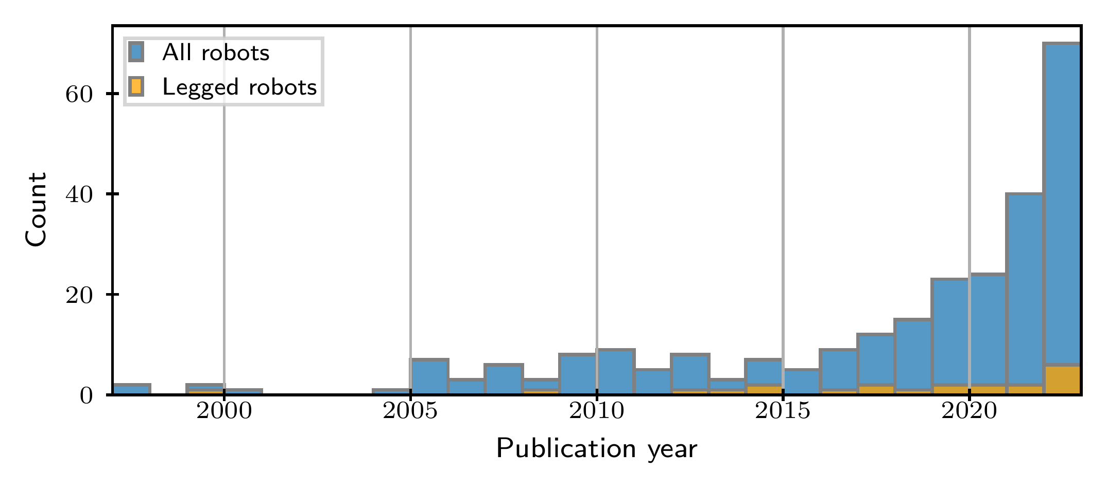
In previous results on legged system co-design, the actuator model and energy efficiency has often been neglected.
Either working with simplified models and or fixating a-priori in the task.
Considering the advancements in the field, we aim of bypassing these limitations.
Can actuator and size of robotic systems be optimized with co-design?
Can energy efficiency be improved for a achieving a specific task?
Once $\color{purple}{\mathcal{D}}$ if fixed, it becomes a standard Optimal Control Problem

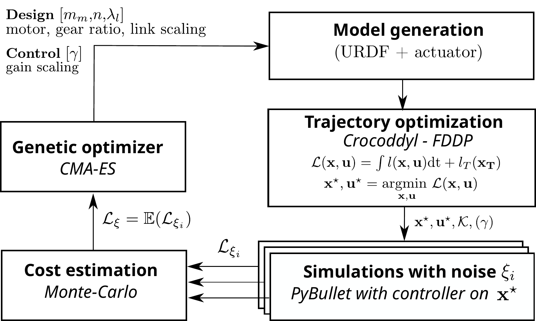
Split the problem with bi-level optimization over design and trajectory

Split the problem with bi-level optimization over design and trajectory
The Robot Model
|
|
|
|
|
|
|
|
|
|
|
|
|
|
|
|
|
|
|
|
|
|
|
|

|
|
|
|


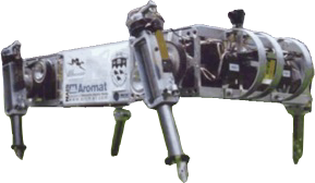
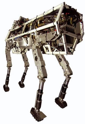
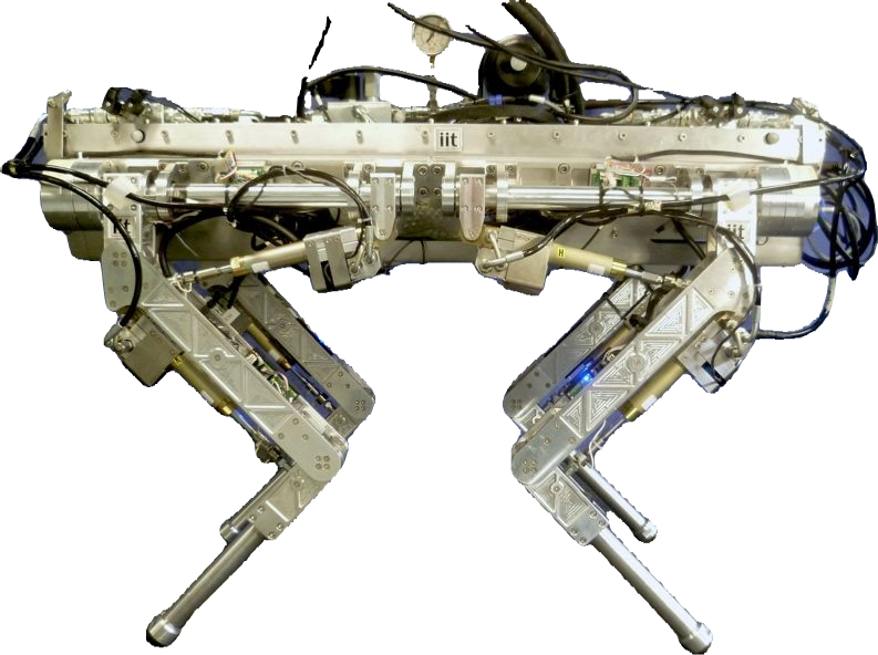
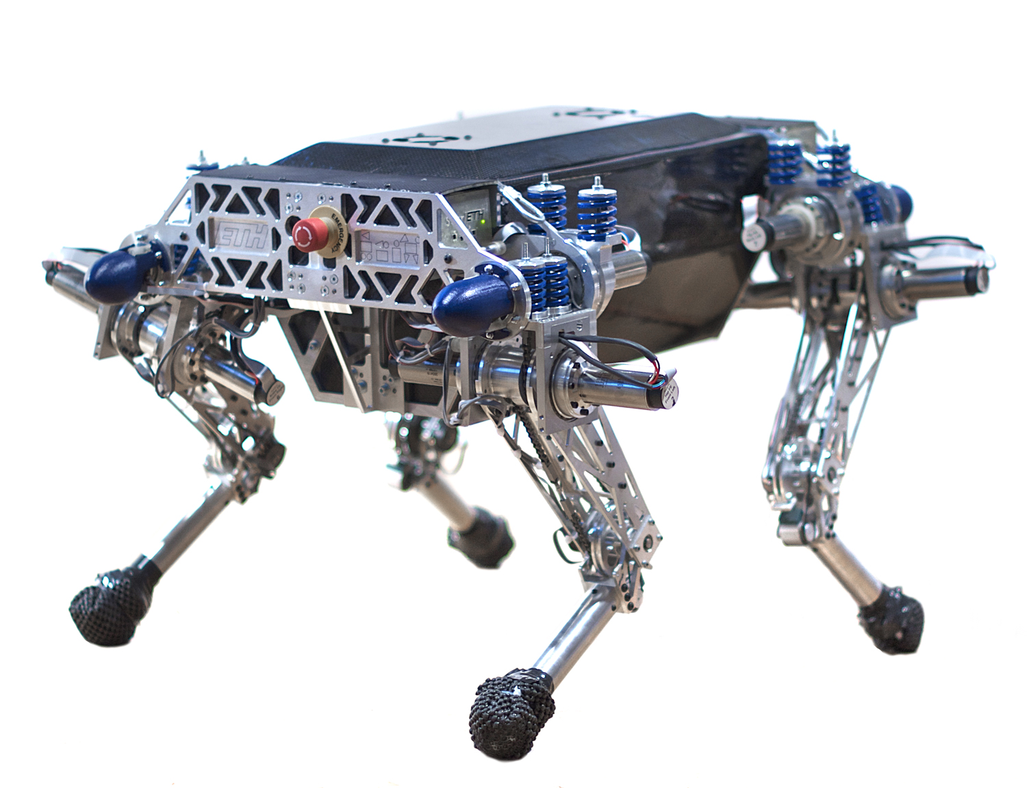
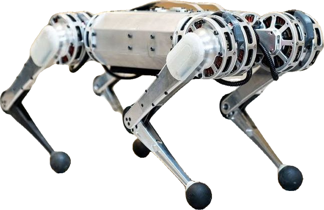
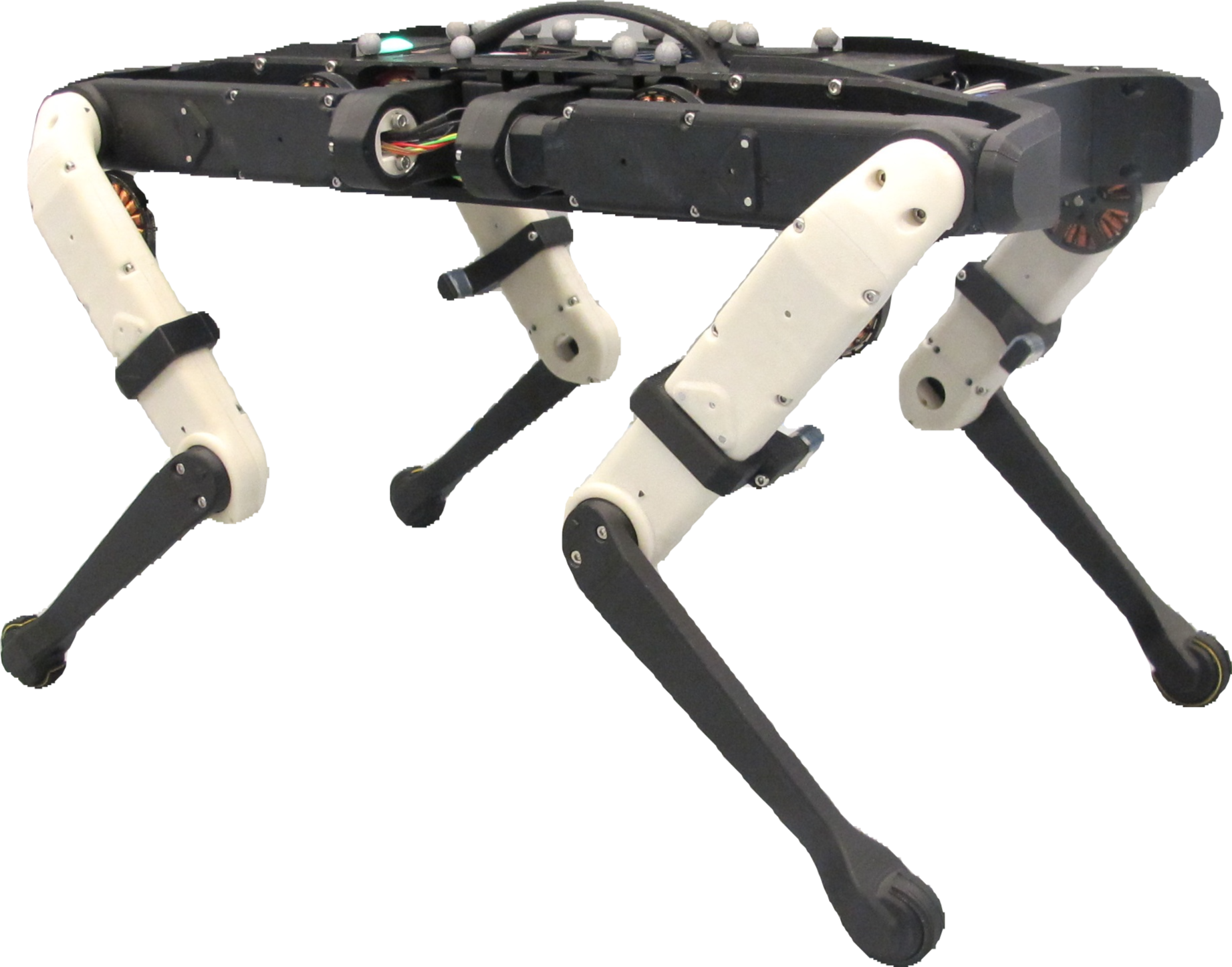
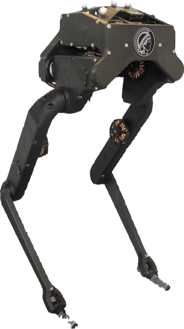
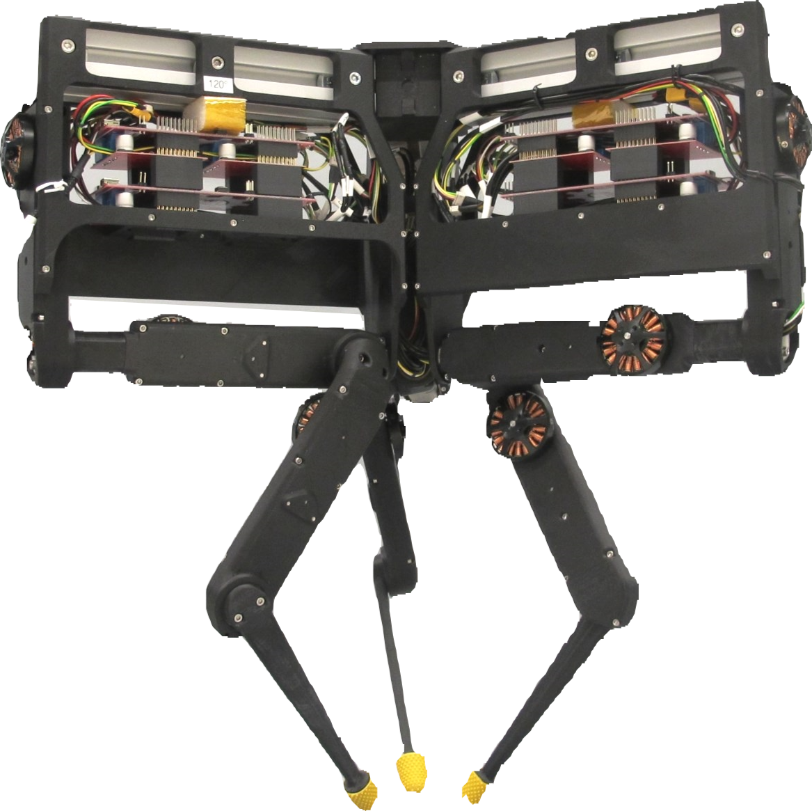
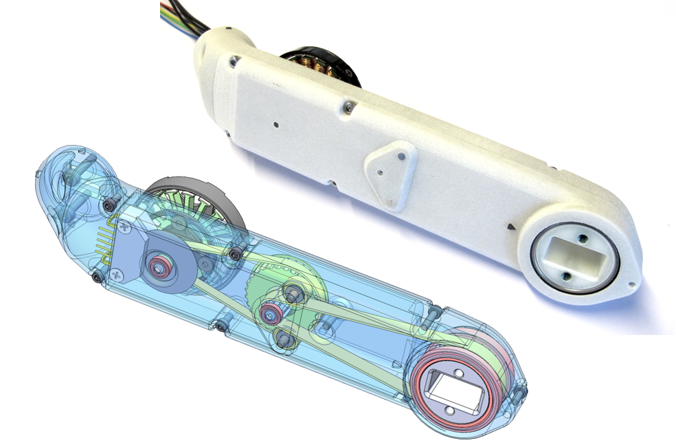
To implement advanced intelligent behaviors several design approaches can be adopted, one of the most promising is the proprioceptive approach1
- Lightweight
- Inertia concentrated in the main body
- High power density QDD
- Back-drivable
To implement advanced intelligent behaviors several design approaches can be adopted, one of the most promising is the proprioceptive approach1
- Lightweight
- Inertia concentrated in the main body
- High power density QDD
- Back-drivable

Develop an optimization strategies to design legged systems for
specific tasks considering their energy efficiency
Link scale modification from a nominal design:
- Structure scaling
- Inertia modification
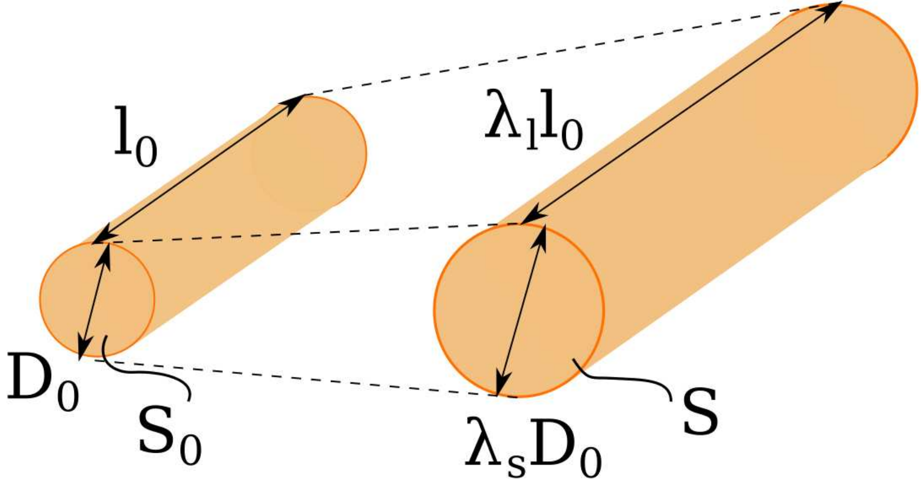
The section of each link is modified so to guarantee structural integrity

Scaling of:
-
$\lambda_l$ link length
-
$\lambda_s$ section
Keeping the normalized deflection constant yields a conservative relationship \[ \lambda_s = \lambda_l^{\frac{3}{2}} \]
So the impact of the length modification is expressed as a function of $\lambda_l$ only
- Motor non-ideality
- Transmission losses
- Friction
- Electro-mechanical coupling
- Inertia
- Added mass to the system
- Rotor inertia
- Electro-mechanical coupling
- Actuator limits
- Max speed
- Max torque
- Bandwidth
Interpolation of the motors properties from dataset


Trajectory Optimization
Minimize electrical power consumption $\color{orange}{P_{el}}$ under dynamic, path constraints.
\[ \begin{aligned} \displaystyle \operatorname*{{minimize}}_{\boldsymbol{x}, \boldsymbol{u}} & \sum_{0}^{N-1} \color{orange}{P_{el}}(\boldsymbol{x}_k, \boldsymbol{u}_k) \text{dt} + \mathcal{L}_f(\boldsymbol{x}_{N}) \\ \mbox{subject to} & \begin{array}{c} \qquad \mathbf{x}_{k+1} = \color{green}{\boldsymbol{\Phi}}(\boldsymbol{x}_k, \boldsymbol{u}_k)\\ \color{blue}{h}(\boldsymbol{x}_k, \boldsymbol{u}_k) \leq 0\\ \end{array} \end{aligned} \]
\[ \begin{aligned} \displaystyle \operatorname*{{minimize}}_{\boldsymbol{x}, \boldsymbol{u}} & \sum_{0}^{N-1} \color{orange}{P_{el}}(\boldsymbol{x}_k, \boldsymbol{u}_k) \text{dt} + \mathcal{L}_f(\boldsymbol{x}_{N}) + \color{blue}{\mathcal{L}_h}(\boldsymbol{x}_k, \boldsymbol{u}_k) \\ \mbox{subject to} & \begin{array}{c} \qquad \mathbf{x}_{k+1} = \color{green}{\boldsymbol{\Phi}}(\boldsymbol{x}_k, \boldsymbol{u}_k)\\ \mbox{} \end{array} \end{aligned} \]
The problem is solved with Crocoddyl1 through Differential Dynamic Programming (DDP)2.
Constraints $\color{blue}{h}$ are relaxed into penalties $\color{blue}{\mathcal{L}_{h}}$ which include:
- Actuator limits (torque, joint velocity, joint position)
- Non penetration
 |
 |
|---|
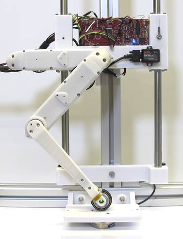
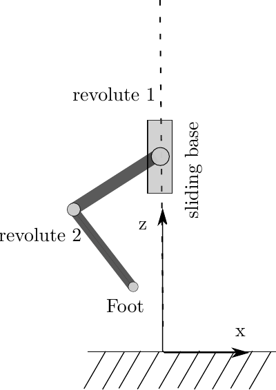
Monoped testbed1
In this approach was implemented for a monoped hopper. Task involves a jump with a re-orientation of the leg to the top in a given amount of time $T=1s$.
| Variable | Range |
|---|---|
| Motor mass $\boldsymbol{m}_m$ | $[0.05, 1]$ kg |
| Gear ratio $\boldsymbol{n}$ | $[3, 20]$ |
| Scaling of the links $\boldsymbol{\lambda}_l$ | $[0.8, 1.2]$ |
| Contact timing $T_c$ | $[0.2s, 0.8]$ s |
| Type | Cost component | Value |
| Terminal cost | Final state | 5e3 |
| Running costs | Power | 2 |
| Torque bounds | 1e1 | |
| Ground contact | 1e6 | |
| Ground | 1e3 |
Design and timing
\[ \begin{cases} m_m &= 9.85 \cdot 10^{-2}[\text{kg}]\\ n &= 4.5\\ \boldsymbol{\lambda}_l &= [0.83, 0.99]\\ T_c &= 0.729\text{s} \end{cases} \]| Type | Nominal | Design | Design and timing |
|---|---|---|---|
| Mechanical Energy | 0.96 J | 1.32 J | 1.47 J |
| Joint friction | 0.87 J | 1.60 J | 0.38 J |
| Joule dissipation | 4.37 J | 1.87 J | 0.53 J |
| Total | 6.19 J | 4.79 J | 2.38 J |
Energy optimal design is found.
Task efficiency can be increased even further by optimizing hyper-parameters, such as the contact timing.
- Co-design framework is applied to a benchmark case.
- A model for the actuator characteristics is proposed.
- Scaling is optimized.
- Result show a great improvement in energy efficiency.
"Computational design of energy-efficient legged robots: Optimizing for size and actuators"
Gabriele Fadini , Thomas Flayols , Andrea del Prete , Nicolas Mansard , Philippe Souères
IEEE International Conference on Robotics and Automation (ICRA 2021)
But what happens when the robot is subject to un-modelled noise?
Can we make sure that the robot can still perform the task under uncertainty?
Can trajectories be tracked even when undergoing external perturbations?
Can the design mitigate the impact of disturbances?
T. Geijtenbeek, et al., Flexible Muscle-Based Locomotion for Bipedal Creatures, ACM ToG
Related to co-design, few approaches have been developed in the past to deal with controller robustness
- Robustness as property of the trajectory, no closed-loop1
- Closed-loop stability metric, sensitivity analysis2,3
- Stochastic optimization, does not scale favourably with the number of scenarios4,5
Optimizing the controller is computationally costly for high-dimensional sytems.
DDP provides a local linear feedback controller via the Riccati gains1.
Stabilizing feeback gains from DDP \[ \delta u = -Q_{uu}^{-1}Q_u - \underbrace{Q_uu^{-1}Q_{ux}}_{\mathcal{K}} \delta x \] Feedback control policy \[ u(x) = u^{\star} + \gamma \mathcal{K} (x - x^{\star}) \]
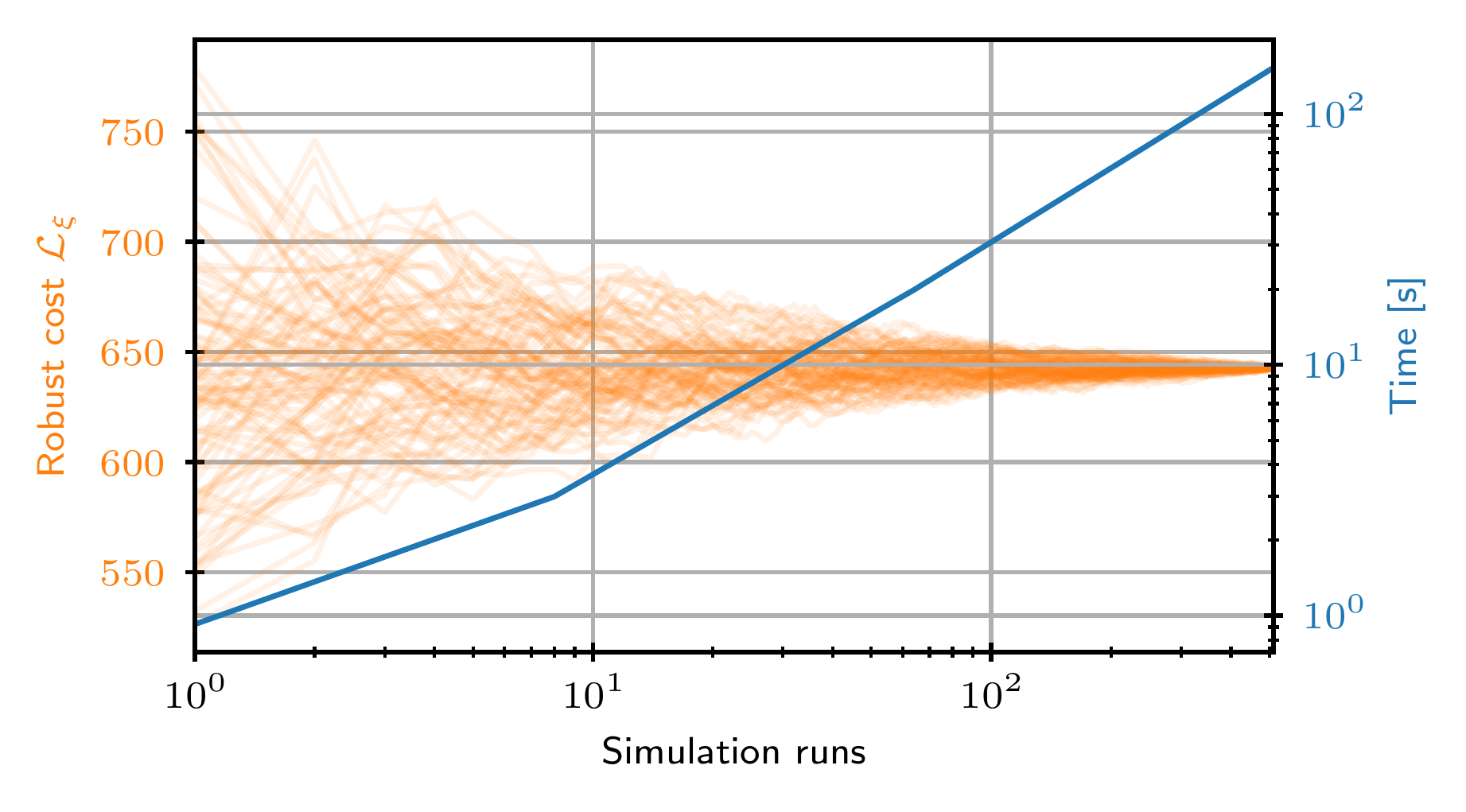
Such controller is used in thousands of perturbed simulations in an approach similar to domain randomization.
Perturb each simulation with $\xi_{i} = \mathcal{N}(0, \sigma_u)$.
Evaluate the cost on the simulated trajectories $x_{\xi,i}, u_{\xi,i}$
\[ \mathcal{L}_\xi = \mathbb{E}(\mathcal{L}_{\xi,i}) = \dfrac{1}{N_{sim}}\sum_{i=0}^{N_{sim}-1} \mathcal{L}(x_{\xi,i}, u_{\xi,i}) \]

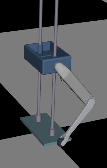
Monoped: underactuated
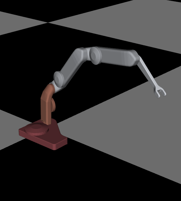
Serial manipulator
- Lightweight and transparent actuators are chosen.
- Robustness is achieved for a small trade-off
- Control parameters (gain scaling) can be optimized.
- Solution can be tested before system integration.
"Simulation aided co-design for robust robot optimization"
Gabriele Fadini , Thomas Flayols , Andrea Del Prete , Philippe Souères
IEEE Robotics and Automation Letters, 2022
Can this bi-level optimization scheme be applied to
more complex problems and robotic systems?
Can we consider different tasks in the optimization?
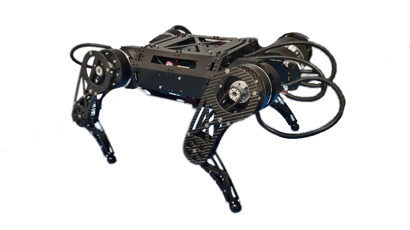
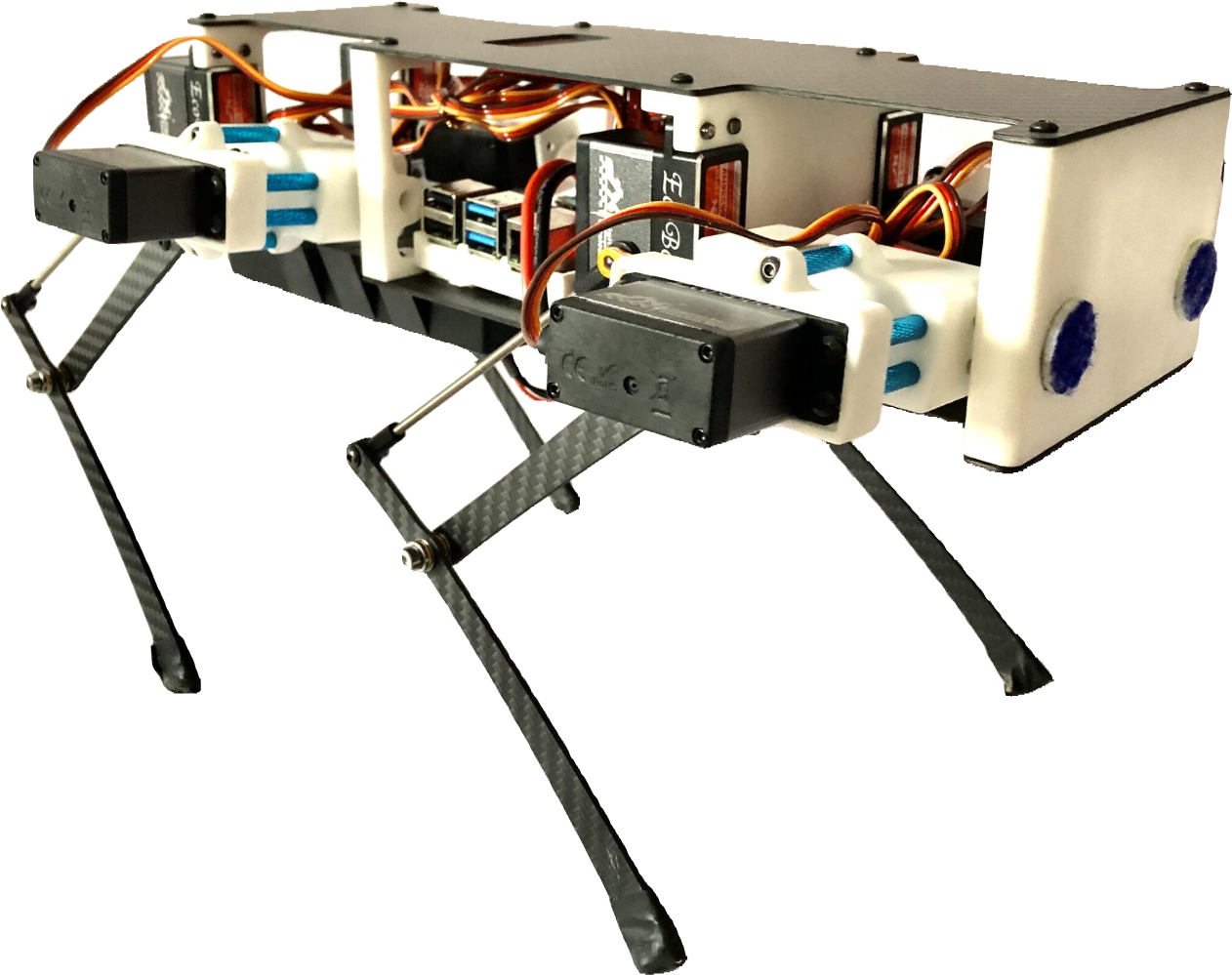
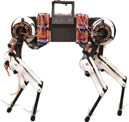
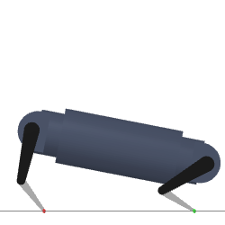
Prototype
Off-shelf motors
In collaboration with

The aim is to to co-optimize a quadruped robot, starting from the prototype (left), based on a open-source project https://mjbots.com/
- Increase its energy efficiency
- Generate cyclic motion patters
- Optimize scale and actuators
Minimize electrical power consumption $\color{orange}{P_{el}}$ under dynamic, path and cyclicity constaints.
\[ \begin{aligned} \displaystyle \operatorname*{{minimize}}_{\boldsymbol{x}, \boldsymbol{u}, \boldsymbol{f}, \boldsymbol{a}, \boldsymbol{\gamma}} & \sum_{0}^{N-1} \color{orange}{P_{el}}(\boldsymbol{x}_k, \boldsymbol{u}_k) \text{dt} + \mathcal{L}_f(\boldsymbol{x}_{N}) \\ \mbox{subject to} & \begin{array}{c} \mathbf{x}_{k+1} = \color{green}{\boldsymbol{\Phi}}(\boldsymbol{x}_k, \boldsymbol{u}_k, \boldsymbol{f}_k, \boldsymbol{a}_k, \boldsymbol{\gamma}_k)\\ \color{blue}{h}(\boldsymbol{x}_k, \boldsymbol{u}_k) \leq 0\\ \color{purple}{g}(\boldsymbol{x}_0, \boldsymbol{x}_N) \leq 0\\ \end{array} \end{aligned} \]
$\color{blue}{h}$ are now hard constraints.
$\color{purple}{g}$ include non-Markov constraints
The resulting NLP is coded in Casadi1 via symbolic expression out of Pinocchio2.
 +
+
Complex behaviors can be produced respecting the actuator bounds
Periodic trajectories are of interest because:
- Limit cycles arise from optimal locomotion1,2,3
- Better reflect continuous operation
Complex behaviors can be produced respecting the actuator bounds
A bounding trajectory was obtained with for the current prototype iteration.
The trajectories are used to validate the power consumption and actuator models.
Optimal energy trajectory can be replayed on the systems with a PD+ controller.
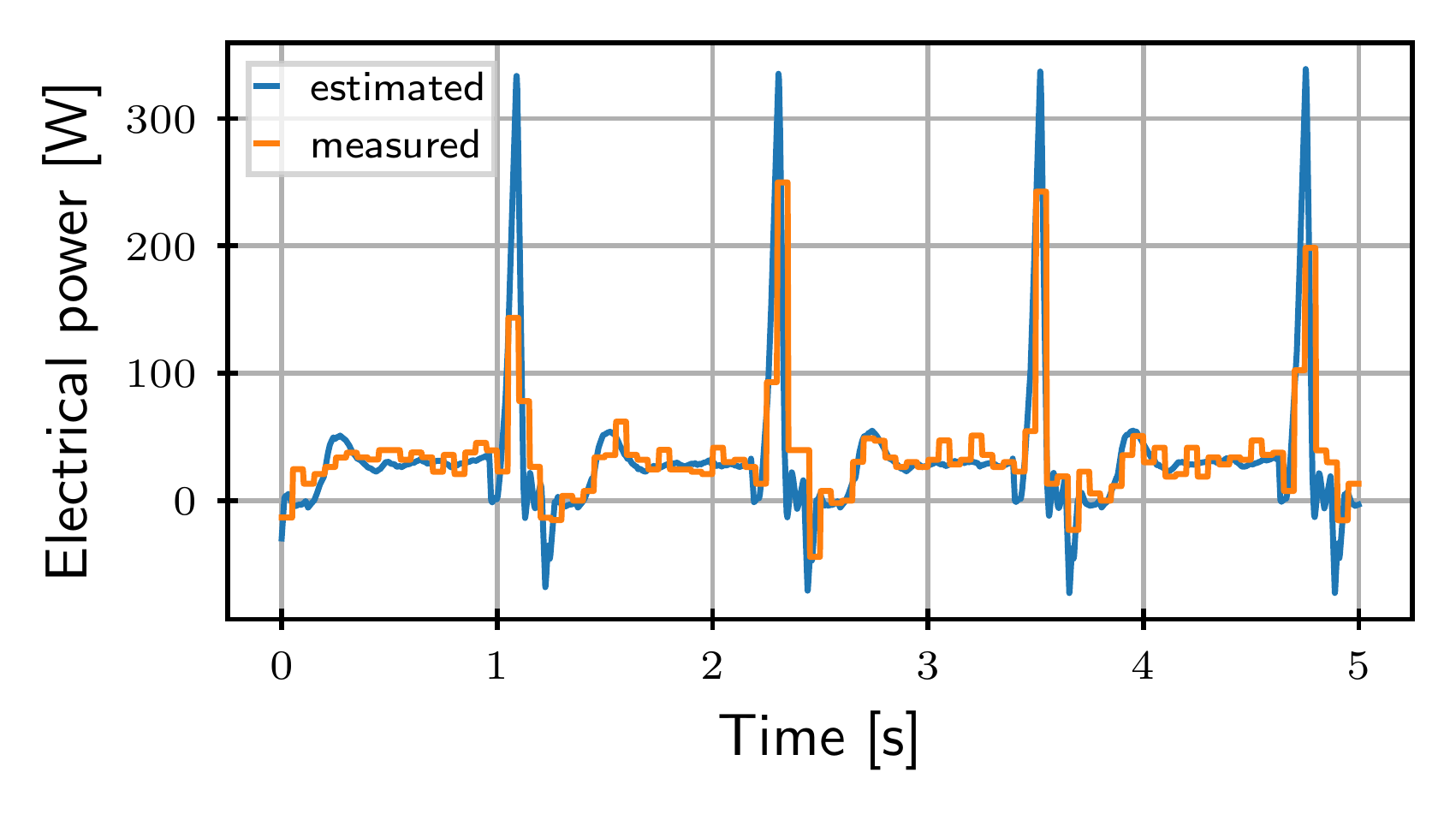
The power consumption model is providing accurate estimates with respect to the measurements data.
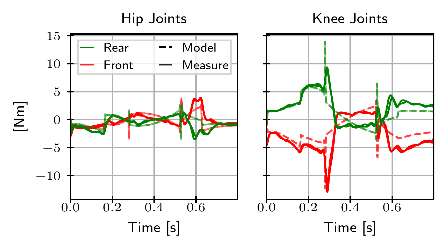
The friction model used in trajectory optimization closely estimates the real torque on the controlled joints.
| Case | Measured | Reference |
|---|---|---|
| Optimal | 39.69 J | 39.64 J |
| Heuristic | 56.75 J | 68.47 J |
With respect to the energy optimal trajectories, the ones obtained
with the heuristic (producing a similar base displacement in a similar amount of time)
are found to be more demanding.
After validation, among possible motions,
bounding and backflip were selected as benchmark behaviors
for co-design.
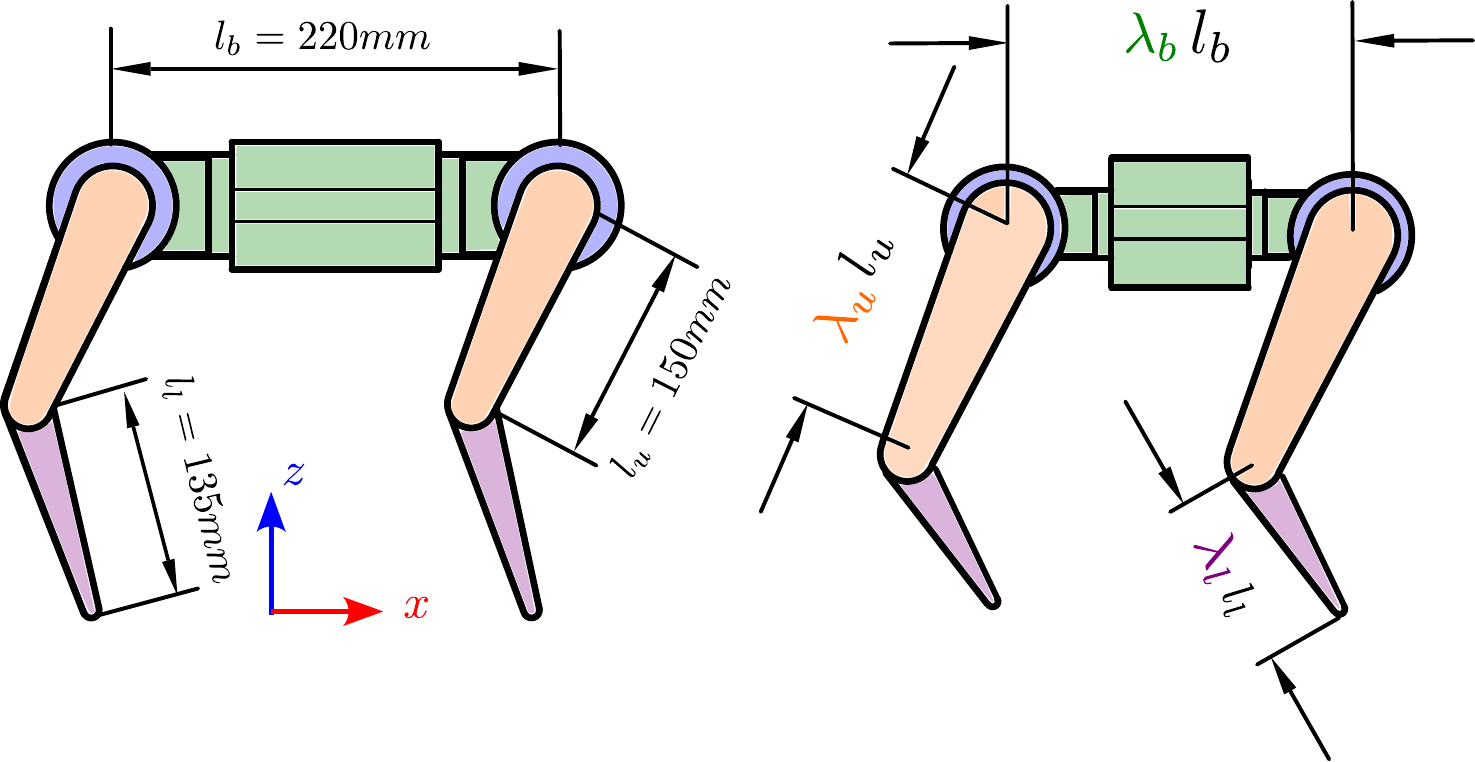
Scaling of the planar model
-
Structure scale:
- base $\lambda_b$,
- thigh $\lambda_u$,
- shank $\lambda_l$
Friction and electro-mechanical properties Actuator limits
-
Motor selection is discrete
- AK80-6
- AK80-9
Energy optimal cyclic trajectories are computed for thousands of designs, changing model, constraints and cost function accordingly selecting the best performing hardware.
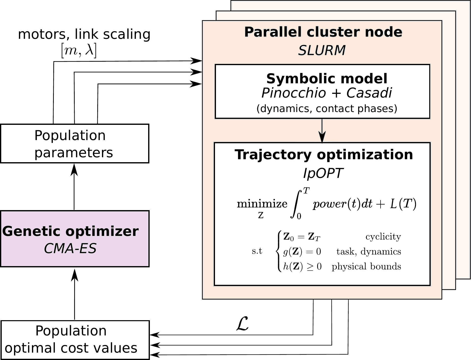
Pallelized HPC framework
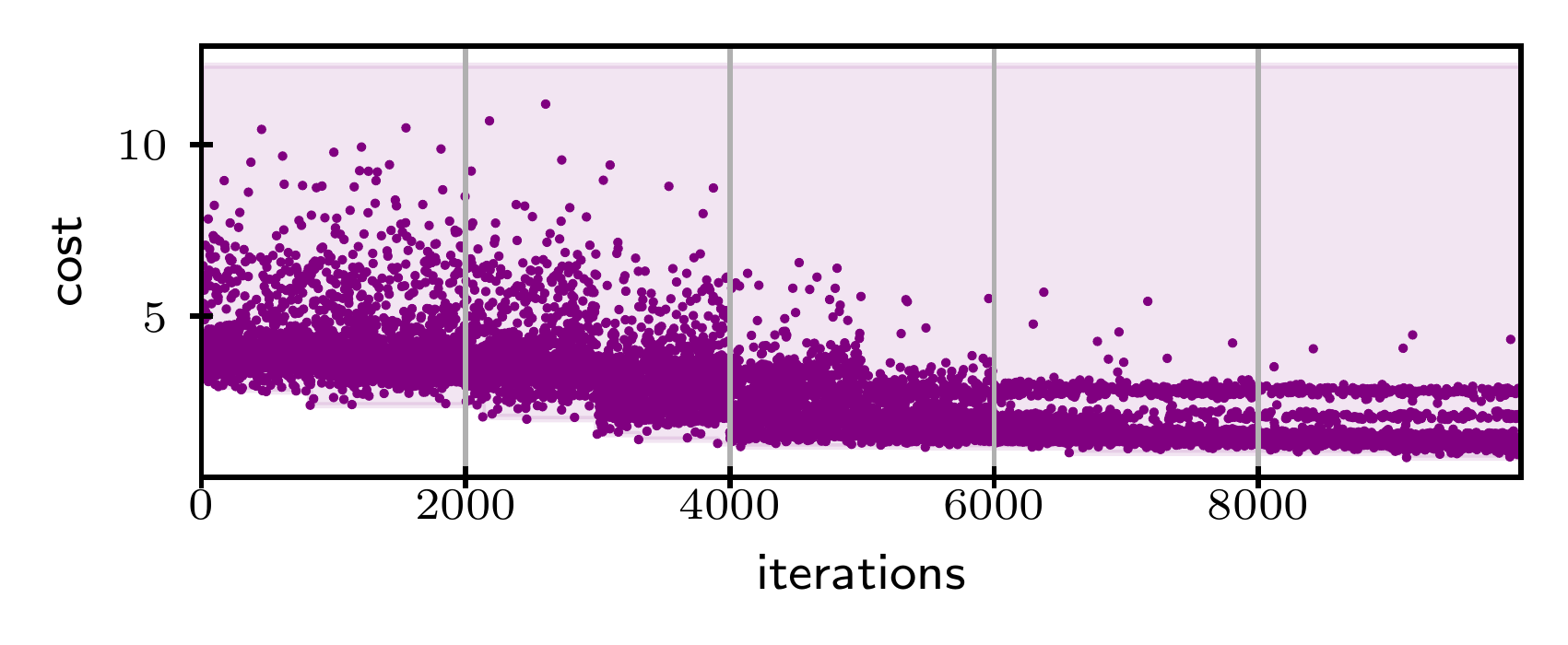
Cost convergence along the optimization
The same design optimization procedure is used for a backflip.
Task: a full base rotation is needed, the state is cyclic except for the rotation and x-translation.
For replayability the robot additionally has zero joint velocity at the begin of the trajectory.
Optimal designs for each of the two chosen tasks are found to be very different among each other.
Best Backflip
$\lambda_b = 1.07$
$\lambda_l = 0.69$
$\lambda_u = 0.50$
$-87\%$
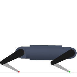
$\leftarrow$ Nominal $\rightarrow$
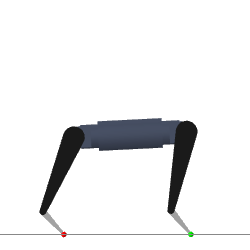
Best Bounding
$\lambda_b = 0.512$
$\lambda_l = 0.514$
$\lambda_u = 0.752$
$-76\%$
As optimization found opposite designs, we looked for a
compromise,
the cost landscapes of the two tasks were
reconstructed keeping the base fixed.
The trade-off is explored fixing $\lambda_b = 1$
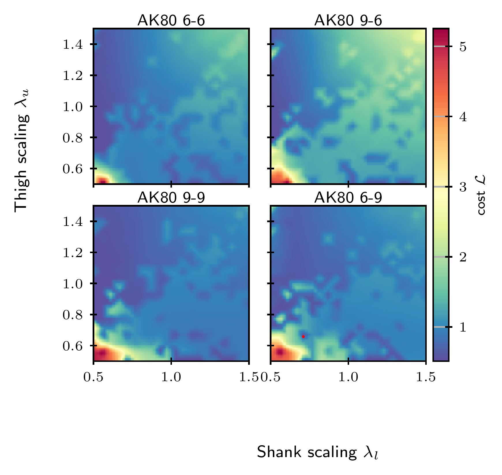
Bounding
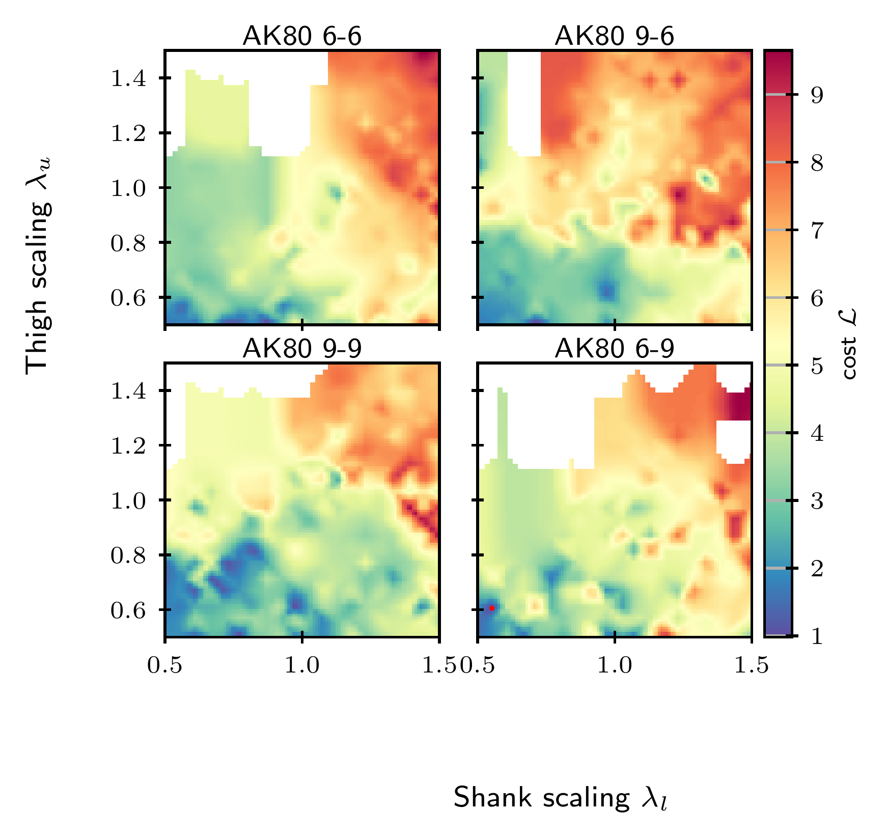
Backflip
+
$\rightarrow$
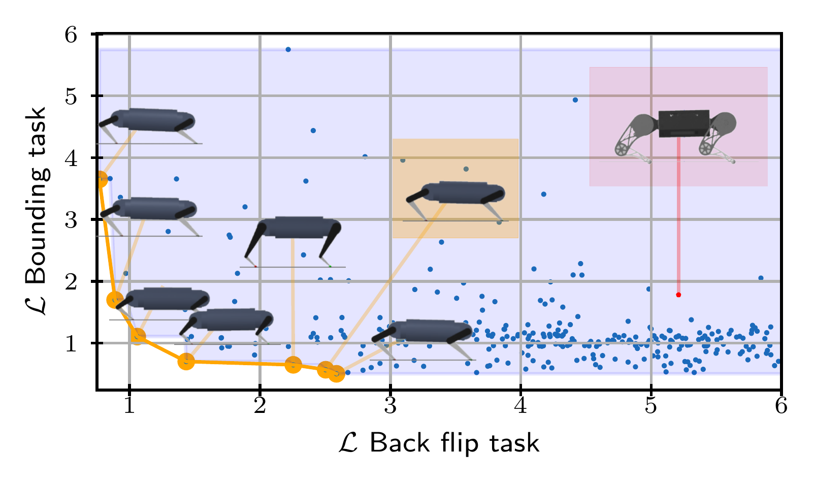
A set of Pareto optimal candidates is found.
| $\lambda_u$ | $\lambda_l$ | $m_{hip}$ | $m_{knee}$ | $\mathcal{L}$ Backflip | $\mathcal{L}$ Bounding |
|---|---|---|---|---|---|
| 0.50 | 0.87 | 6 | 6 | 1.06 | 1.11 |
| 0.50 | 1.03 | 6 | 6 | 2.59 | 0.5 |
| 0.66 | 1.03 | 6 | 6 | 2.5 | 0.57 |
| 0.61 | 0.55 | 6 | 6 | 0.77 | 3.65 |
| 0.50 | 0.71 | 9 | 9 | 0.89 | 1.70 |
| 0.61 | 0.97 | 9 | 9 | 1.43 | 0.70 |
| 1.08 | 0.50 | 9 | 9 | 2.26 | 0.65 |
The trade-off is selected and energy efficiency is improved up to $50\%$ for both tasks.
-
Validation of the actuator model and trajectories on a real system
-
Modification of the framework to be more general and robust
-
Strategy to handle discrete variables
-
Multiple cyclic tasks are optimized
"Co-designing versatile quadruped robots for dynamic and energy-efficient motions"
Gabriele Fadini , Shivesh Kumar , Rohit Kumar , Thomas Flayols , Andrea Del Prete, J. Carpentier, P. Soueres
2023, submitted to Robotica, preprint available
The presented results show:
- Optimization for energy-optimal trajectories and design is possible.
Hardware is selected based on a rich dynamic model, with the actuator and scaling. - Power minimization provides accurate estimates and replayable trajectories.
-
Useful findings are systematically recovered.
Energy efficient designs are found to be lightweight and exploit at best the plant dynamics.
- The approach is versatile and can be used on several systems and tasks.
-
The approach, used for simple problems, shows that optimizing hardware for several task is possible.
Further generalization is necessary to cope with the complexity of both the system and task.
-
Trajectory optimization is computationally expensive and requires expert knowledge.
It could be made more efficient by using data.
Behaviour synthesis could be automatized with Reinforcement Learning.

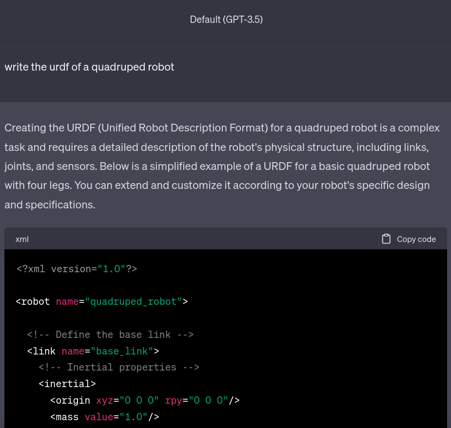
What is the robot DNA? Going toward fully specifying the robot mechatronic design. Implementation and validation on hardware still require further refinement from the designer. A more complete robot specification encoding needs to be developed.
How far can we go with robot automatic design generation?
Design generation could be automatically learned, still user knowledge and intuition should be integrated in co-design. This process of learning user preferences could be obtained in a similar way to model refinement to Large Language Model.
There is still some work to do, but maybe we are on the right track.

Thanks for your attention
- F. Grimminger et al., "An Open Torque-Controlled Modular Robot Architecture for Legged Locomotion Research", IEEE RAL, vol. 5, no. 2, April 2020
- M. Bogdanovic, et al. "Learning Variable Impedance Control for Contact Sensitive Tasks", RAL, vol. 5, issue 4, 2020
- K. Mombaur. “Using optimization to create self-stable human-like running”, Robotica 2009.
- P. Robuffo et al. “Trajectory Generation for Minimum Closed-Loop State Sensitivity”, ICRA 2018.
- P. et al. Brault. “Robust Trajectory Planning with Parametric Uncertainties”, ICRA 2021.
- I. et al. Mordatch. “Ensemble-CIO: Full-body dynamic motion planning that transfers to physical humanoids", IROS 2015.
- G. Bravo Palacios, et al. “One Robot for Many Tasks: Versatile Co-Design Through Stochastic Programming", RAL 2020.
- E. L. Dantec, et al. "First Order Approximation of Model Predictive Control Solutions for High Frequency Feedback", RAL 2022.
Extra Slides
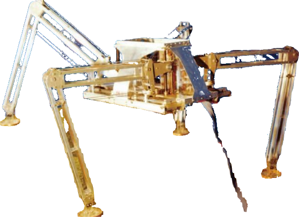
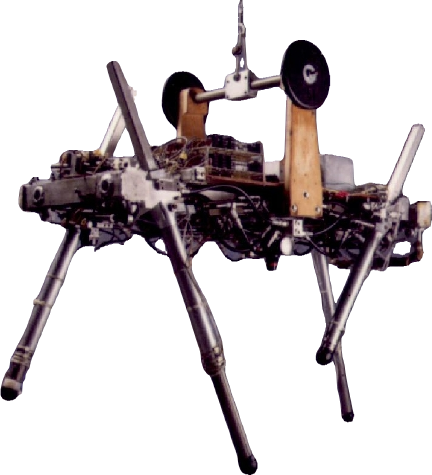
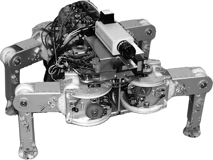
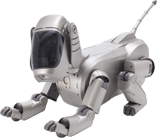
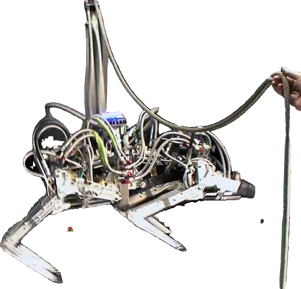
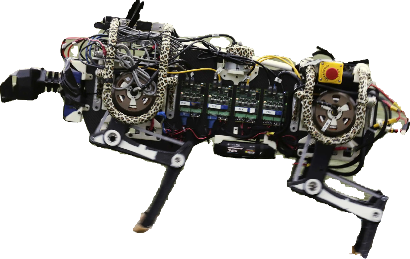
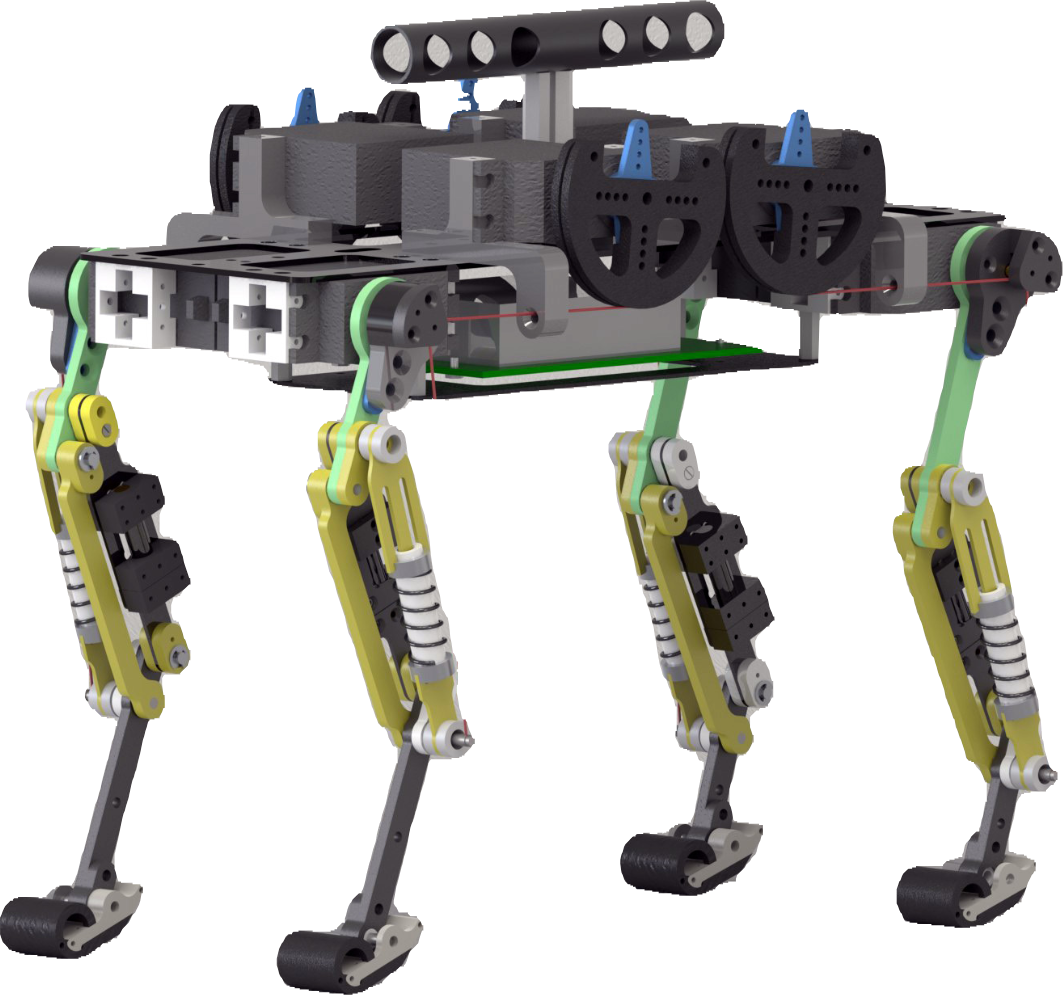
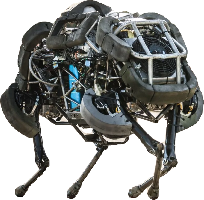
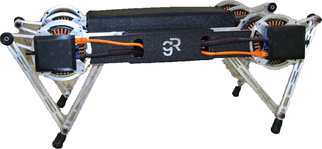
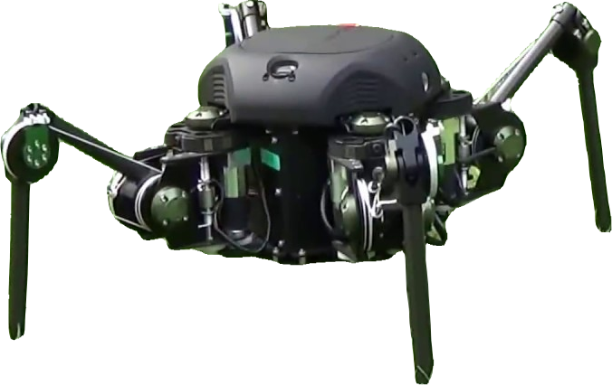
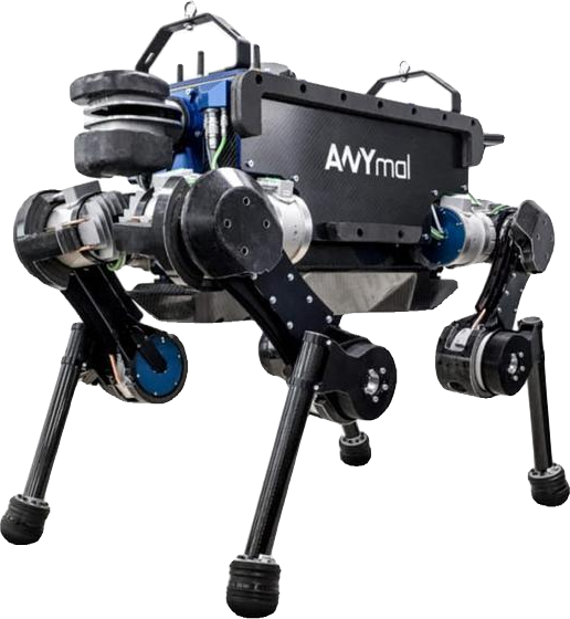
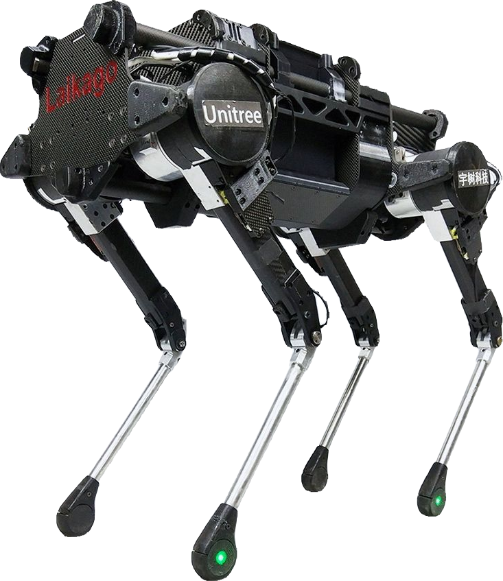
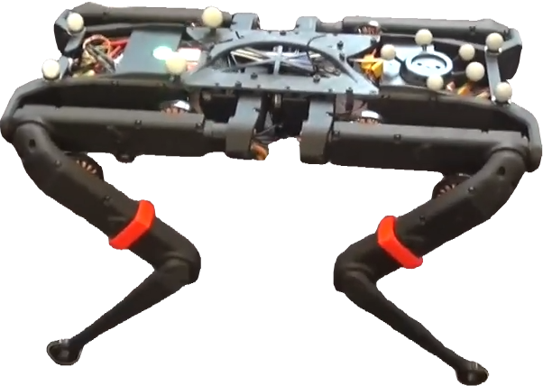
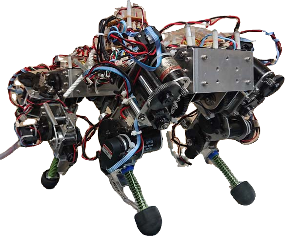
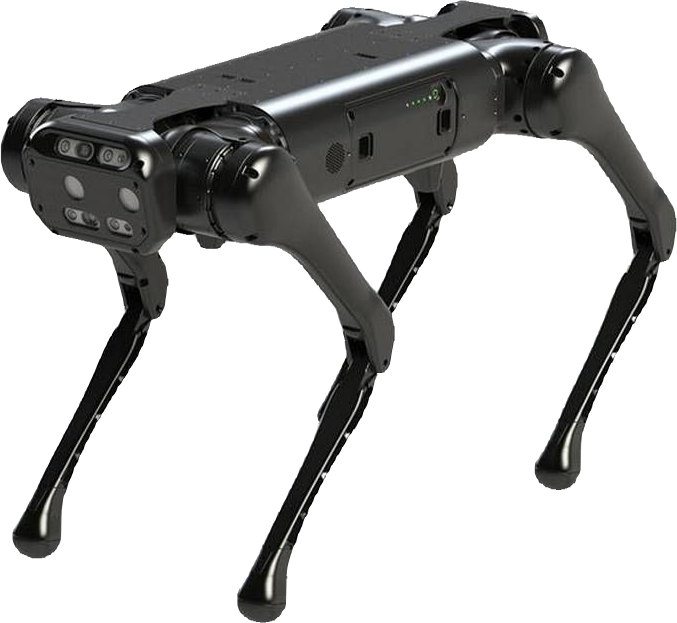
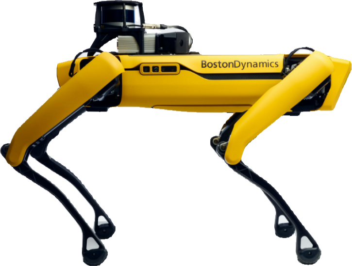
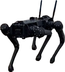
Successful robot embody
an intelligent design
- ATLAS
- Digit
- MiniCheetah
- Solo
- Anymal
| Quantity | Robust | Standard |
| Cost $\mathcal{L}$ | $\color{orange}{9.58\text{e}-3}$ | $\color{green}{3.5\text{e}-3}$ |
| Cost $\mathcal{L}_{\xi}$ | $\color{orange}{33.42}$ | $\color{red}{2\text{e}3}$ |
| $\lambda_l$ | $[0.83, 1.02, 0.86]$ | $[0.80, 0.80, 1.08]$ |
| $m_m$ | $\color{green}{[0.05, 0.05, 0.05, 0.06]}$ | $\color{orange}{[0.2, 0.76, 0.49, 0.4]}$ |
| $n$ | $[16.7, 11.6, 11.8, 15.2]$ | $[17.1, 11.8, 11.4, 15.3]$ |
| RMSE | $0.287$ | $1.836$ |
| $\sum_{i}P_{m,i}{dt} \;[J]$ | $-0.9$ | $-1.7$ |
| $\sum_{i}P_{t,i}{dt} \;[J]$ | $\color{red}{6.5}$ | $\color{green}{1.8}$ |
| $\sum_{i}P_{f,i}{dt} \;[J]$ | $\color{green}{1.3}$ | $\color{orange}{3.2}$ |
Results for the manipulator back and forth task optimization
